One of the basic properties of numbers is that they may be expressed in exponential form. We are all familiar with the representation 1000 = 103 or 0.001 = 10-3. A more general way of stating this property is to say that any number (N) may be expressed as a base (B) raised to a power (x) or
In the examples above the formula the base is 10. Further examples using
base 10, base 2, and base e (where e = 2.718...) are given below in Table
1.
|
|
|||||
| Number = 10x | Number = 2x | Number = ex | |||
| .01 | 10-2 | 1 | 20 | .01 | e-4.605 |
| 1 | 100 | 2 | 21 | 1 | e0 |
| 10 | 101 | 4 | 22 | 10 | e2.303 |
| 1000 | 103 | 8 | 23 | 1000 | e6.908 |
| 2 | 10.301 | 2 | e.693 | ||
| 4 | 10.602 | 4 | e1.386 | ||
| 8 | 10.903 | 8 | e2.079 | ||
The first four entries in the base-10 section look natural as do the entries in the base 2, but few students would immediately guess .301 as the appropriate exponent for 2 = 10x. Further, the natural base e (e = 2.71828..) probably seems at first an illogical base for representing numbers. As will be discussed below, exponential functions of the type y = aebx are very common in describing physical and chemical systems, and a basic understanding of this type of function is necessary.
The mathematical statement N = Bx serves as the basis for defining logarithms. The logarithm of a number (N) in base (B) is defined as (x).
logarithm(B)N = x
Two bases, 10 and e, are in common usage. The shorthand representations are:
base 10 logarithm10 N = log10 N = log NThus, the logarithm of a number is simply the power to which the base must be raised to give the number. Table 2 shows the log and ln of the numbers in Table 1.
and
base e ("Natural" logarithms) logarithme N = ln N
|
|
||
|
|
|
|
|
|
|
|
|
|
|
|
|
|
|
|
|
|
|
|
|
|
|
|
|
|
|
|
|
|
|
|
NOTE:
Only the numbers to the right of the decimal point in a logarithm are
significant figures. The number to the left of the decimal point simply,
in effect, tells us where the decimal point is and is not considered a
significant figure.
There are a few basic rules for handling logarithms. Examples are given in base 10 but the rules are applicable to any base.
Rule 1:
log (a x b) = log a + log b
Examples:
log (2000) = log (2 x 1000) = log 2 + log 1000 = .301 + 3 = 3.301Rule 2: log (a/b) = log a - log b
log (.004) = log (4 x .001) = log 4 + log .001 = .602 - 3 = -2.398
Examples:
log (2/4) = log 2 - log 4 = .301 - .602 = -.301Rule 3: log (a)b = b log a
log (2/.4) = log 2 - log .4 = log 2 - [log (4 x .1)] = .301 - [.602 - 1] = .699
Examples:
log (4)3 = 3 log 4 = 3 x .602 = 1.806Rule 4: log (10)x = x
log (8)1/2 = 1/2 log 8 = 1/2 x .903 = .452
Examples:
log 10-8 = -8If one has the logarithm of a number and wishes to find the number, one simply raises the base to the power of the logarithm. This is called taking the antilogarithm.
ln e4 = 4
Examples:
antilog .301 = 10.301 = 2Note: On most calculators, antilogarithms may be taken by
antilog 1.806 = 101.806 = 64
antilog -2.398 = 10-2.398 = .004
antiln 2.303 = e2.303 = 10
antiln 1.386 = e1.386 = 4
While logarithms are interesting and useful in their own right, they have greatest applicability for us in dealing with exponential functions.
- INV + log or INV + ln
or- 10x or ex
or- yx where y = BASE.
One of the very common functional relationships appearing from experimental observations is that of an exponential increase or decrease. This takes the form of an expression as
y = ex and y = e-x
In the more general form this appears as
y = eax and y = e-ax
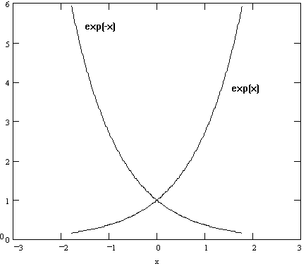
where a groups together any quantities that can be considered to be constant during the variation of x and y. When graphed, these functions appear as seen in Figure 1 (note that when x = 0, y becomes = 1). Base e logarithms can be converted to base 10 logarithms.
Figure 1. Exponential Functions
Since it is very difficult to obtain the exact form of the coefficient
a from graphs such as these, it becomes more convenient to apply logarithms
to functions in this form. Thus,
y = eax becomes ln y = ax; y = 10a'x becomes
log y = a'x
or 2.3 log y = ax. [Note that a' = a/2.3 ]
and a plot of ln (or log) y versus x will then give a straight line whose slope will be "a." The same considerations apply to these expressions when they are straight lines as to any straight line.
In a simple case, consider the data from Table 3 for the decomposition
of hydrogen peroxide. Two ways in which these data can be graphed are shown
below: (a) concentration against time on rectangular coordinates, (b) log
concentration against time on rectangular coordinates. These are illustrated
in Figures 2a - 2b.
|
Decomposition of Hydrogen Peroxide |
||
| Time | Concentration | Log Concentration |
|
|
|
|
|
|
|
|
|
|
|
|
|
|
|
|
|
|
|
|
Figure 2a. Decomposition of Hydrogen Peroxide
Plot of Concentration vs Time
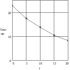
Figure 2b. Decomposition of Hydrogen Peroxide
Plot of log Concentration vs Time
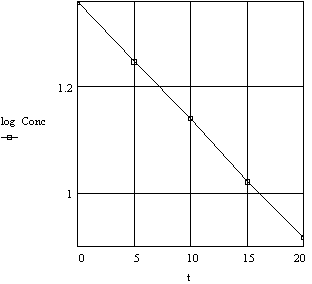
Whether one uses the logarithmic or exponential form for such relationships depends on what is to be determined. Mathematically the exponential form has certain advantages while graphically the logarithmic form is more informative. Any functional relationship in this form has recognizable characteristics that are more obvious when one more symbol is included in the general expression. Thus,
y = yoe-ax
where yo is a constant determined by the fact that when x = 0, the value of e-ax = 1 and under these conditions, y = yo. The following examples illustrate the general characteristics of this type of function. The "a" is a specific constant in each example.
- The decrease in the concentration of reacting material c per unit time t is proportional to the concentration and is expressed as
- The decrease in the intensity of the incident light, I, is proportional to the depth, l, of the absorbing material and is expressed as
- The pressure of the atmosphere P decreases at a rate proportional to the altitude h and is expressed as
c = coe-at
where co is the concentration at time t = 0 (at the beginning of the experiment).
I = Ioe-al
where Io is the intensity of the incident radiation at l = 0, before it passes through the absorbing material.
P = Poe-ah
where Po is the pressure at h = 0, sea level.
- Plot the given numerical values for x and y on a piece of graph paper using y as the vertical axis (ordinate) and x as the horizontal axis (abscissa). If a graphing program for a microcomputer is available, it provides a convenient way go examine a graph without resorting to a paper copy. The experimentally independent value is generally put on the x axis, and the experimentally measured, dependent, variable on the y axis.
- If the resulting plot shows a straight line, the equation for the original numerical values is easily determined since the equation of a straight line is
y = mx + b
where m = slope and b = intercept of line with y axis (at x=0).
slope = m = rise/run = 2/3
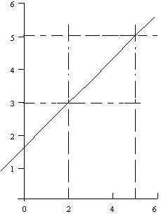
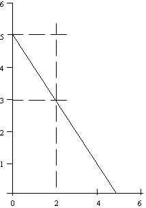
Figure B. Negative slope
slope = m = rise/run = -2/2 = -1
- If the plot resulting from step I is not a straight line, you are not particularly likely to happen on the equation by inspection. I.e. the fact that if x = 3, y = 9, (a single point) does not imply that the equation is y = x2 (holds for all points). One method is to convert the original data to a straight line. In this course we will encounter several relationships of the form
Calculate or read off the values for m and b, then insert the m and
b values into the equation y = mx + b. The result should be the equation
you're looking for. To double check your work, try some of the original
given values for x in your equation and see if y comes out as expected.
The equation of the line in Fig. A is y = 2x/3 + 5/3 and for Fig. B is
y = -x + 5 = 5 - x.
y = ae-b/T
where y is some property of the system, a and b are constants and T is the temperature in Kelvins. These functions are all linearized by taking the natural logarithym of the expression.
ln y = ln a - b/T. A plot of ln y vs 1/T will give a straight line with slope -b and intercept ln a.
| Density | Temperature |
| (g/mL) | (degrees C) |
|
|
|
|
|
|
|
|
|
|
|
|
|
|
|
|
|
|
|
|
|
|
|
|
||
|
|
||
|
|
||
|
|
||
|
|
||
|
|
||
|
|
||
|
|
||
|
|
||
|
|
||
(a) y = 3x2 + 4
(b) y = 3e2x
(c) y = 6e-4x
(d) y = 3e4/x
(e) y = 2e-8/x
D = -2.5 x 10⁻³ T + 13.60
|
|
|
|
|
|
|
|
|
|
|
|
|
|
|
|
|
|
|
|
|
|
|
|
|
|
|
|
|
|
|
|
|
|
|
|
|
|
|
|
|
|
|
|
|
|
|
|
|
|
|
|
|
|
|
|
|
|
|
|
|
|
|
|
|
|
|
|
| (d) |
|
|
|
|
|
|
|
|
|
|